Moonfrog Labs uses Amazon Redshift to analyze mobile game telemetry. Each session, purchase, and player drop-off generates events that product and analytics teams use to understand game performance. Faster loading and querying help those teams work with fresher data.
Moonfrog runs a single production analytics cluster with roughly 148 TB in Amazon Redshift Managed Storage (RMS) and about 4,000 warehouse tables. It also queries roughly 1,000 external data lake tables. The warehouse supports telemetry ingestion, revenue reporting, marketing attribution, and self-service dashboards for product, data science, analytics, and support teams.
In this post, we show how Moonfrog migrated its production analytics warehouse from Amazon Redshift RA3 to RG instances using elastic resize. We explain how the team selected capacity for growing analytics demand and more frequent loading, verified warehouse and data lake access, and assessed performance and costs after migration.
The challenge
Moonfrog’s RA3 cluster ran reliably, with no stability issues. Its constraint was compute headroom as analytics demand grew. Ingestion volume was steady before migration. Growth came from analytical queries and data lake scans. The team already planned to expand from five RA3 nodes to six or seven nodes and wanted capacity to load warehouse data more frequently.
The five-node ra3.4xlarge cluster averaged about 54% CPU utilization. In approximately 98% of hours, CPU peaked at or above 90%. Other indicators showed demand increasing:
- SELECT queries per day increased 31% from January to July.
- Mean workload management (WLM) queue wait for highest-priority queries rose from 505 milliseconds in May to 940.7 milliseconds in July.
- Concurrency scaling usage nearly doubled over the same period, from 4,453 to 8,516 seconds per day.
A COPY operation averaged 16.8 seconds on RA3. That duration constrained how often the stats pipeline could load. The team evaluated RG as a way to support growing analytics demand and make more frequent loads practical.
Moonfrog also queried roughly 1,000 external tables in Amazon Simple Storage Service (Amazon S3). Data scanned through Redshift Spectrum increased 33%, from 84.9 TB in March to 112.5 TB in June. The separate Spectrum scanning charge added to the cost of expanding RA3 compute.
Moonfrog used WLM query monitoring rules to stop scans larger than one terabyte. These rules controlled scan spend under the RA3 configuration.
The one-year no-upfront reserved node commitment for ra3.4xlarge expired in July 2026. Renewal gave Moonfrog an opportunity to re-evaluate its compute commitment and determine whether switching to RG would provide additional headroom for its growing workload needs.
Solution overview
Amazon Redshift RG instances use AWS Graviton processors and an integrated data lake query engine. AWS publishes benchmarks of up to 2.2 times faster warehouse workloads and up to 2.4 times faster Apache Iceberg workloads, at 30% lower price per vCPU than RA3. These benchmarks are separate from Moonfrog’s production results. RG runs Apache Iceberg and Apache Parquet scans on cluster nodes, removing the separate per-terabyte Spectrum charge for these scans. Elastic resize supports changing the node family and capacity without a customer-managed export and reload.
Moonfrog retained its ingestion and analytics architecture at cutover. No service was added or removed, and applications continued to use the same warehouse.
The following diagram illustrates the architecture.
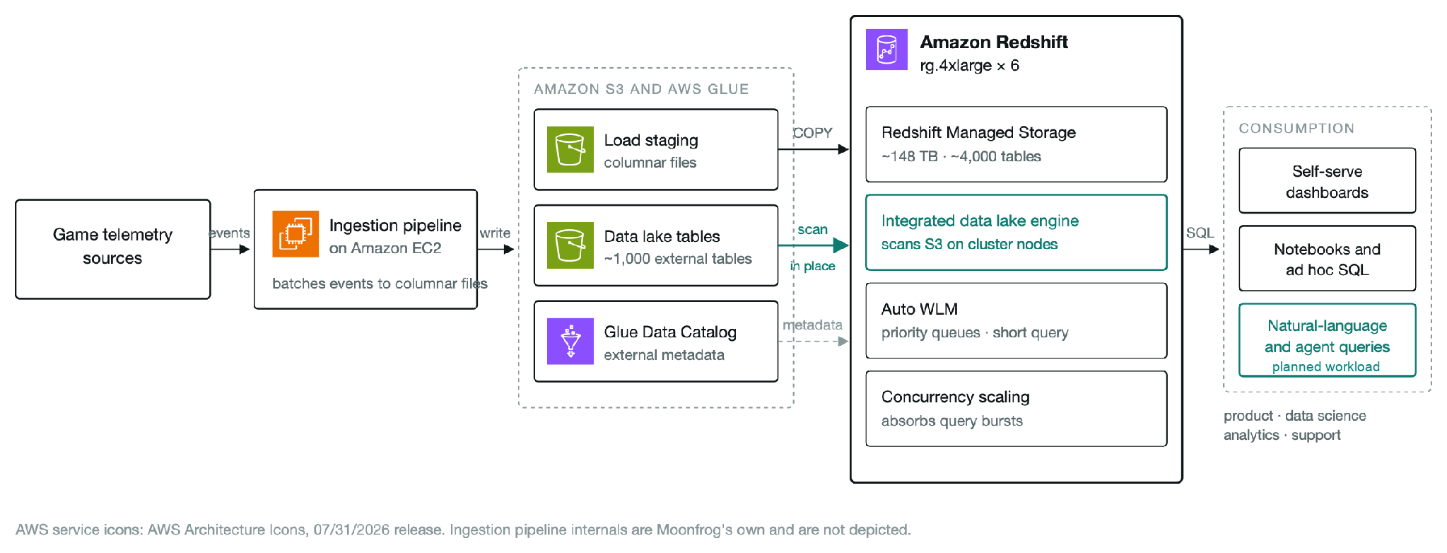
Figure 1: The ingestion pipeline writes columnar files to Amazon S3. COPY loads warehouse tables, and the integrated data lake engine on RG queries external tables in place. Conversational analytics is a planned use of the additional headroom
The architecture uses the following AWS services:
- Amazon Redshift provides the analytics warehouse and integrated data lake engine.
- Amazon S3 stores event files, load staging data, and external data lake tables.
- AWS Glue Data Catalog stores metadata for external schemas and tables.
- Amazon Elastic Compute Cloud (Amazon EC2) runs the ingestion pipeline.
- Amazon CloudWatch and AWS Cost Explorer provide performance and billing measurements.
Implementation steps
Moonfrog established a baseline, used elastic resize to change the node family, and verified warehouse and data lake access. It then evaluated the early results before selecting its final configuration.
Step 1: Establish a baseline
Before the change, the team captured Amazon CloudWatch metrics for CPU utilization, WLM queue wait by priority, query duration by type, and queries per day. COPY loads and SELECT queries were measured separately. Billing records provided reserved compute, Spectrum scanning, and concurrency scaling costs so the comparison covered each billing line affected by the move.
AWS provides migration planning and workload validation guidance in the AWS RA3 to RG best practices blog.
Step 2: Validate the target configuration and use elastic resize
AWS recommends testing the target RG configuration in a non-production environment with representative workloads before migrating production. That testing is intended to measure benefits, identify issues, and validate the target size before the production migration.
On 26 July, Moonfrog used elastic resize to move from five ra3.4xlarge nodes to eight rg.4xlarge nodes, temporarily providing extra capacity to reduce migration risk. It did not export or reload the 148 TB warehouse. Schemas, ETL jobs, application SQL, drivers, connection strings, and BI tools continued to work.
Amazon CloudWatch recorded one five-minute interval in which the cluster reported unhealthy. Database connections recovered immediately afterward. This sampling interval describes the observed impact. It does not establish an exact five-minute outage duration.
AWS guidance describes elastic resize as a short operation, typically about 10 to 15 minutes. After an RA3-to-RG node-type change, data hydration brings frequently accessed data from managed storage into the new nodes’ local cache. This cache warming should be considered when interpreting early performance measurements.
Step 3: Verify warehouse and data lake access
Moonfrog verified that warehouse loads and external queries continued after the resize. External schemas and tables remained in use, with AWS Glue Data Catalog providing their metadata.
Moonfrog confirmed that per-terabyte S3 scanning charges were eliminated for its RG queries in the subsequent billing records. Those queries used provisioned cluster capacity, which remained billable.
Step 4: Review workload management rules
Moonfrog’s Auto WLM configuration included separate queues for administrators, analysts, ETL, loading, and visualization, along with short query acceleration. These queues carried across the migration. The team reviewed query monitoring rules because data lake scans now consumed RG cluster capacity.
The review accounted for data lake scans sharing compute with warehouse workloads. Rules that previously controlled scan spend could still protect these shared resources.
Results and key benefits
The following four CloudWatch charts cover 1 May to 25 October 2026. Each marks the 26 July resize and shades the 26 July–3 August period when the cluster was reduced from eight to seven to six RG nodes. Query duration and WLM wait charts show seven-day rolling means. Query counts include COPY, SELECT, INSERT, utility, and other operations.
Stage 1: Evaluate RG after cutover
The first evaluation focused on workload continuity and query runtime. Warehouse loads and data lake queries continued, and the applications used the same schemas, SQL, drivers, and connection strings. Queries on the initial RG configuration were completing within expected runtimes. Moonfrog then reduced the node count in stages to assess whether each reduction affected query runtime.
The cleanest comparison of COPY duration is 27–31 July, when load volume remained unchanged. Mean duration fell from 16.8 seconds on RA3 to 3.6 seconds on RG, about 79% shorter. This window falls within the 26 July–3 August right-sizing period, before the final six-node configuration was established.
Select six nodes
Moonfrog reduced the cluster from eight to seven and then six RG nodes within eight days. The team retained the additional node relative to its five-node RA3 baseline to support growing analytical demand and more frequent loading. It had already planned to expand RA3 to six or seven nodes.
The move from five RA3 nodes to six RG nodes increased node count by 20%. Published node specifications list 12 vCPUs per ra3.4xlarge and 16 per rg.4xlarge, so provisioned vCPUs increased from 60 to 96, or 60%. The results reflect the change in both node family and capacity.
Stage 2: Sustain performance as workloads grow
After validating the available headroom on the six-node configuration, Moonfrog increased loading frequency on 24 August. The cluster now executes more than 70,000 COPY operations a day, about 4.3 times the RA3 baseline. These loads use smaller, more frequent batches, so later COPY duration also reflects the changed loading pattern. Figure 2 shows the early duration improvement and subsequent performance as the workload changed.
In late August, after the 24 August increase in loading frequency, Moonfrog purchased a one-year no-upfront reservation for the six-node RG configuration. The purchase followed its evaluation of RG with production traffic and committed capacity for anticipated workload growth.
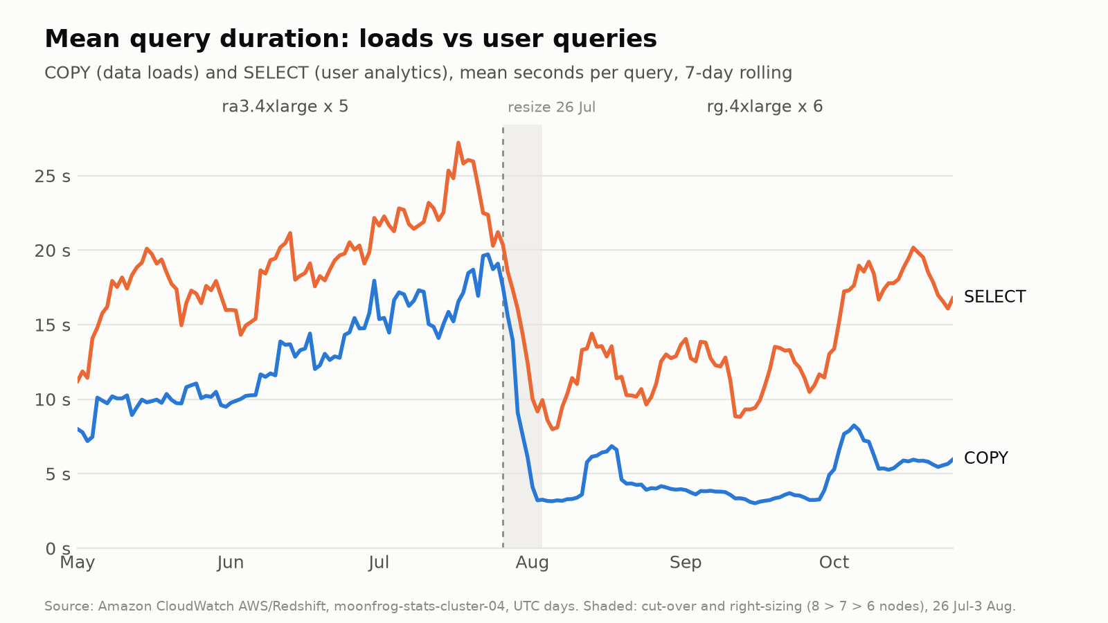
Figure 2: Mean COPY and SELECT duration. The early COPY comparison uses unchanged volume. Later means also reflect smaller batches after 24 August
More daily queries with compute headroom
Daily queries across all types increased from around 49,122 on RA3 to 83,603 in August, 125,350 in September, and 125,374 during 1–25 October. From September onward, this was more than 2.5 times the RA3 baseline. COPY accounts for much of that increase, so total query growth should be read alongside the query mix in Figure 3.
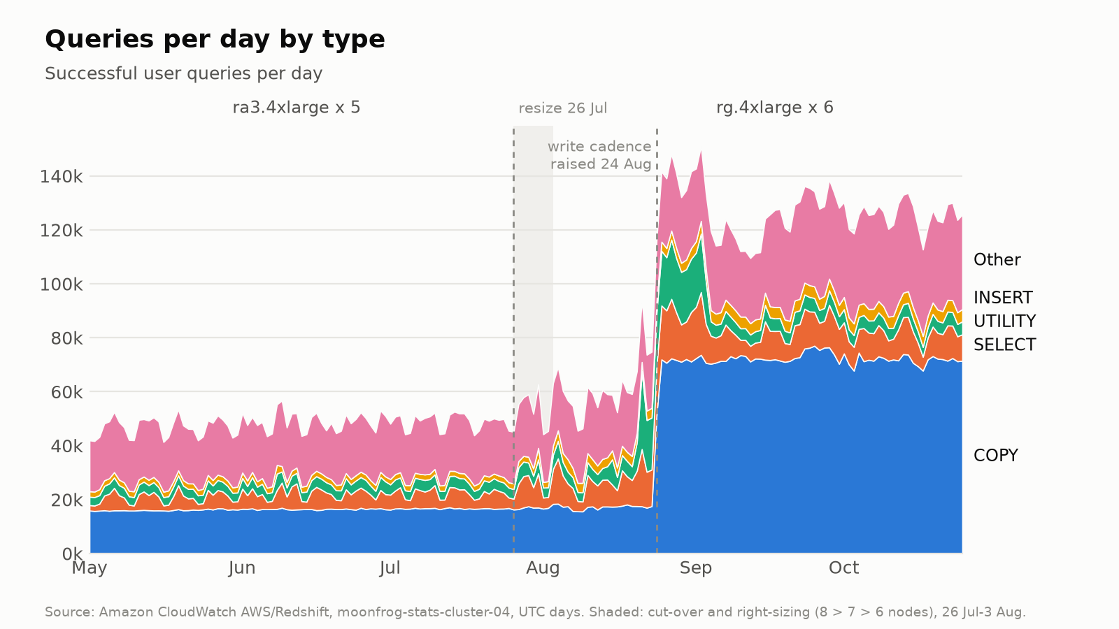
Figure 3: Successful daily queries by type. COPY frequency increased on 24 August, after the migration and right-sizing period
Concurrency scaling remained enabled to absorb peak bursts alongside the six reserved nodes. Average daily usage was 14–29% below the RA3 baseline in August, September, and October, even as total query volume grew. Usage increased from September to October as demand rose.
Average CPU utilization fell from about 54% on RA3 to 35–39% from September onward, despite the higher query count. Figure 4 distinguishes daily average CPU from the typical peak, defined as the daily mean of each hour’s maximum CPU reading.
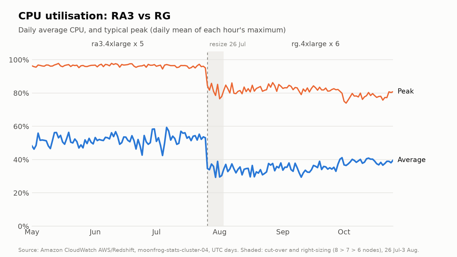
Figure 4: CPU utilization before and after the resize. The typical peak is an average of hourly maximum readings, not the single daily maximum
Queue waits as demand grows
Queue waits fell after migration and rose from their August lows as traffic increased in October. During 1–25 October, highest-priority waits averaged 561 milliseconds versus a July RA3 baseline of 940.7 milliseconds, and high-priority waits averaged 193 milliseconds versus 294 milliseconds. Normal-priority waits were about 11 milliseconds, above their July baseline of about 3.6 milliseconds. Figure 5 uses a separate vertical scale for each priority.
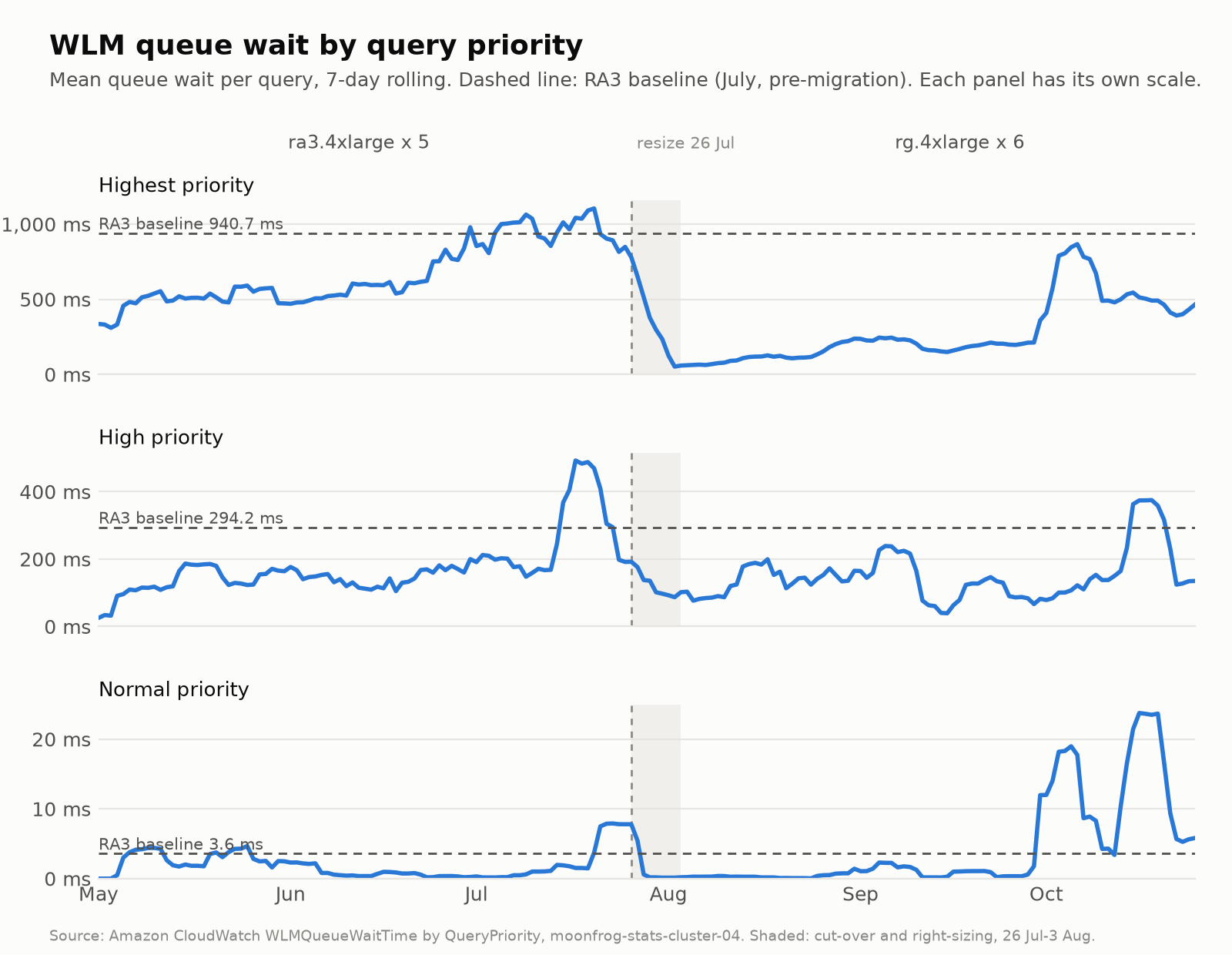
Figure 5: Seven-day rolling mean WLM queue wait by priority. Dashed lines mark July RA3 baselines. Each panel has its own scale
Integrated data lake queries and billing
External data lake queries continued after migration. Moonfrog confirmed that the separate Spectrum scanning charge remained exactly $0 from 27 July through the reported months:
- The Amazon Redshift system views showed that external queries continued. A recent three-day sample recorded roughly 200,000 external queries against Amazon S3, including Parquet scans. External schemas and tables remained in use.
- Billing records showed no separate per-terabyte scanning charge. External scans use provisioned RG capacity, which remains billable. Amazon S3 storage and other charges are outside this comparison.
Cost per query
Moonfrog chose additional capacity for growth, and monthly spend across reserved compute, Spectrum scanning, and concurrency scaling increased approximately 4–6%. On a consistent 30-day basis, cost per 1,000 total queries fell approximately 59% in September and 58% in October. Costs per 1,000 SELECT queries fell 38–50% across August through October.
| Metric | RA3 × 5 Before | RG × 6 August | RG × 6 September | RG × 6 Oct 1–25 |
| Queries per day All types | 49,122 | 83,603 | 125,350 | 125,374 |
| Cost per 1,000 total queries | $5.60 | $3.45 −38% | $2.28 −59% | $2.33 −58% |
| Reported cost per 1,000 SELECT | $45.60 | $22.73 −50% | $25.19 −45% | $28.34 −38% |
Cost per 1,000 total queries is calculated by dividing the combined 30-day spend for reserved compute, Spectrum scanning, and concurrency scaling by 30 times the average daily query count, then multiplying by 1,000. These are aggregate cost measures, not the execution cost of an individual query.
How the team plans to use the headroom
The larger configuration created room to test additional analytical use cases. Earlier measurements showed mean short-query duration falling from about 2.8 seconds to 1.8 seconds. That observation applies to the measured short-query workload and does not establish a response-time guarantee for every analytical question.
Moonfrog plans to evaluate conversational analytics using large language model (LLM) agents. Such agents may execute several queries to answer one question, so query latency is one part of the end-to-end response time. The additional compute headroom gives the team room to test these workloads alongside existing analytics.
Lessons learned
- Use a reserved node renewal as an opportunity to review capacity and architecture for your growing workload needs. Moonfrog evaluated RG before making another one-year commitment.
- Size the cluster for expected workload growth and assess results against the capacity provisioned. Moonfrog added a sixth node for headroom. Interpret total query counts alongside the query mix, because smaller, more frequent COPY batches increase the number of operations.
- Include concurrency scaling in capacity planning. In this deployment it continued to absorb peak bursts alongside the reserved nodes, so evaluate its contribution when assessing warehouse throughput.
- Separate immediate migration results from subsequent workload changes. The unchanged-volume COPY comparison captures the first days after cutover. Later results include the loading cadence change and rising demand. Measure dashboard latency and query abandonment separately to quantify the effect on users.
Next steps
Moonfrog has already increased warehouse loading frequency. The team plans to measure dashboard load times and query abandonment to assess how greater freshness and shorter query durations affect the experience of product and analytics teams.
Moonfrog is considering Apache Iceberg for data lake tables currently stored as Parquet files. The table format would add capabilities such as schema evolution and time travel. The team will evaluate these changes alongside performance and operating requirements.
The team also plans to evaluate broader natural language access. Governance must define which teams can access each table and how exploratory queries share cluster resources. End-to-end agent response time will need separate measurement.
Conclusion
Moonfrog migrated its 148 TB production Amazon Redshift warehouse from five RA3 nodes to RG using elastic resize, then settled on six nodes after eight days of measured right-sizing. RA3 had run reliably. The change addressed growing analytics demand and the need for more frequent warehouse loads. COPY duration fell from 16.8 seconds to 3.6 seconds at unchanged volume immediately after cutover.
With six RG nodes, Moonfrog handled more than 125,000 daily queries across all types from September onward, over 2.5 times the RA3 baseline. Average CPU utilization was 35–39%. More frequent COPY batches contributed to the change in query mix. External queries continued with no separate Spectrum scanning charge, and concurrency scaling provided burst capacity alongside the reserved nodes.
To evaluate RG for your warehouse, review Amazon Redshift pricing, the elastic resize documentation, and the RA3 to RG migration best practices. Establish a baseline and test representative workloads in a non-production environment first. Validate warehouse and data lake access, then compare total spend and cost per unit of work before committing to reserved capacity.